Feature engineering

This is my notes on feature engineering. The idea is to populate this article with all possible relevant knowledge I can get on my hands on and then use it as a reference in the future. Plan is also to use what I Study and note once, use many times.

mindmap
  root((Feature engineering))
    Feature transformation
        Handling missing values
            Imputation
                Remove observation
                Mean replacement
                Median replacement
                Most frequest categorical
        Handling categorical values
            One-hot-encoding
            Binning
        Handling outliers
            Outlier detection
            Outlier removal
        Feature scaling
            Standardization
            Normalization
    Feature construction
        Domain knowledge
        Experience
    Feature selection
        Feature importance 
    Feature extraction

import polars as pl
input_data_path = f"../data/iot/iot_telemetry_data.parquet"
df_original =  pl.read_parquet(input_data_path)
df_original.head(1)

shape: (1, 9)

ts	device	co	humidity	light	lpg	motion	smoke	temp
f64	str	f64	f64	bool	f64	bool	f64	f64
1.5945e9	"b8:27:eb:bf:9d:51"	0.004956	51.0	false	0.007651	false	0.020411	22.7

1. Feature transformation

Importing modules

import duckdb
import polars as pl
import seaborn as sn
import pandas as pd
import matplotlib.pyplot as plt

Reading data

# ts is in epoch time format so converting it to timestamp
# rounding values for temperature and humidity
# converting temperature from farhaneit to celsius
df_raw = duckdb.sql(
    f"SELECT ts, to_timestamp(ts) AS timestamp, device, temp,ROUND((temp - 32) * 5.0 / 9, 4) AS temp_c, ROUND(humidity, 4) AS humidity, lpg, smoke, light FROM '{input_data_path}'"
)

Exploring the data

The seven questions to get insight into the data

How big is the data?

# Converting to polars to easy statistics and exploration
df_original = df_raw.pl()  
df_original.shape

(405184, 9)

Imputation / Handling missing values

This dataset is quiet clean, there are no missing data in the input data in any feature. Docs Reference

df_original.null_count()

shape: (1, 9)

ts	timestamp	device	temp	temp_c	humidity	lpg	smoke	light
u32	u32	u32	u32	u32	u32	u32	u32	u32
0	0	0	0	0	0	0	0	0

Handling categorical variables

Outlier detection

Feature scaling

Datetime transformation

The ts column is in unix seconds, which we will convert to timestamp.

df_original = df_original.with_columns(pl.from_epoch(pl.col("ts"), time_unit="s").alias("timestamp"))
df_original.head(2)

shape: (2, 9)

ts	timestamp	device	temp	temp_c	humidity	lpg	smoke	light
f64	datetime[μs]	str	f64	f64	f64	f64	f64	bool
1.5945e9	2020-07-12 00:01:34	"b8:27:eb:bf:9d:51"	22.7	-5.1667	51.0	0.007651	0.020411	false
1.5945e9	2020-07-12 00:01:34	"00:0f:00:70:91:0a"	19.700001	-6.8333	76.0	0.005114	0.013275	false

What is the date range of the data collected?

The time range of the dataset is

print(df_original.select(pl.col(['timestamp', 'ts'])).describe())

shape: (9, 3)
┌────────────┬────────────────────────────┬───────────────┐
│ statistic  ┆ timestamp                  ┆ ts            │
│ ---        ┆ ---                        ┆ ---           │
│ str        ┆ str                        ┆ f64           │
╞════════════╪════════════════════════════╪═══════════════╡
│ count      ┆ 405184                     ┆ 405184.0      │
│ null_count ┆ 0                          ┆ 0.0           │
│ mean       ┆ 2020-07-16 00:06:56.798528 ┆ 1.5949e9      │
│ std        ┆ null                       ┆ 199498.399262 │
│ min        ┆ 2020-07-12 00:01:34        ┆ 1.5945e9      │
│ 25%        ┆ 2020-07-14 00:20:00        ┆ 1.5947e9      │
│ 50%        ┆ 2020-07-16 00:06:28        ┆ 1.5949e9      │
│ 75%        ┆ 2020-07-18 00:02:56        ┆ 1.5950e9      │
│ max        ┆ 2020-07-20 00:03:37        ┆ 1.5952e9      │
└────────────┴────────────────────────────┴───────────────┘

Find the average humidity level across all sensors.

df_original.select(pl.col("humidity").mean())

shape: (1, 1)

humidity
f64
60.511694

Remove unwanted columns

We are only interested in certain columns, the rest of the columns can be removed.

irrelevant_columns = ["co", "lpg", "motion", "smoke", "ts", "light"]
for columnname in irrelevant_columns:
    pass
    #df = df_original.drop(columnname)
#df_original.head(1)

Reorganize the columns

df = df_original.select(['timestamp', 'device', 'temp', 'humidity'])
df = df.sort(by="timestamp")
df.head(1)

shape: (1, 4)

timestamp	device	temp	humidity
datetime[μs]	str	f64	f64
2020-07-12 00:01:34	"b8:27:eb:bf:9d:51"	22.7	51.0

import seaborn as sn
sn.lineplot(df.head(100), x="timestamp", y="temp")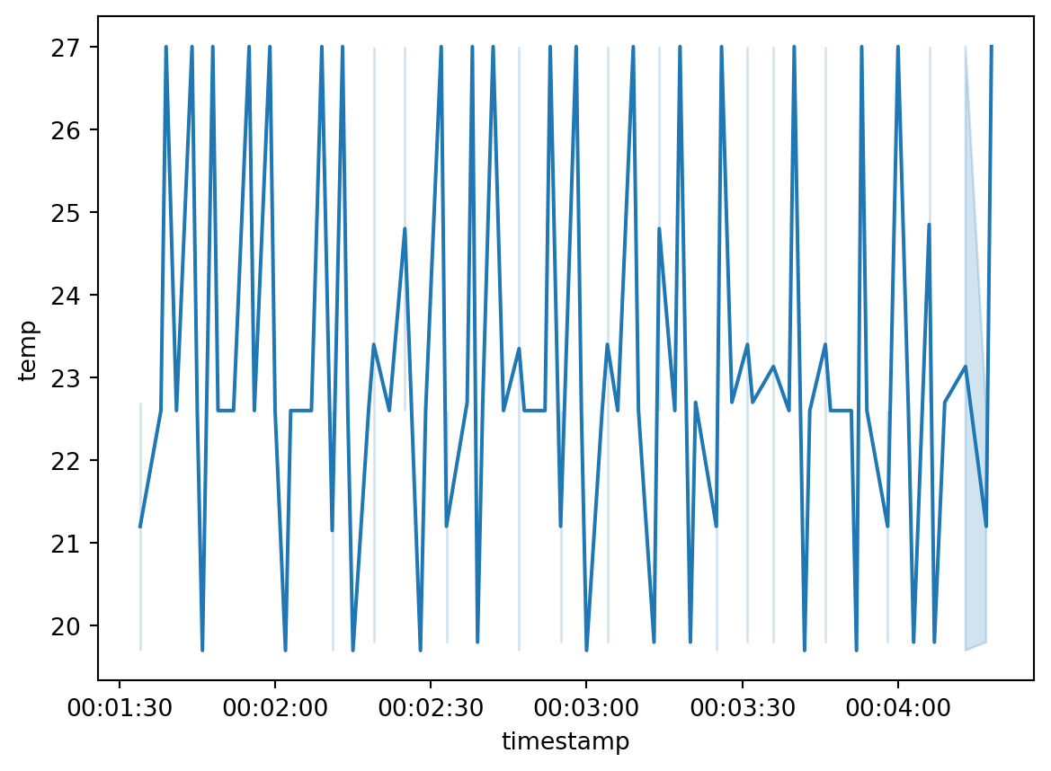

from prophet import Prophet
import pandas as pd
import dyplot
df_device_1 = df.filter(pl.col("device")=="b8:27:eb:bf:9d:51")
df_device_2 = df.filter(pl.col("device")=="00:0f:00:70:91:0a")
df_device_3 = df.filter(pl.col("device")=="1c:bf:ce:15:ec:4d")


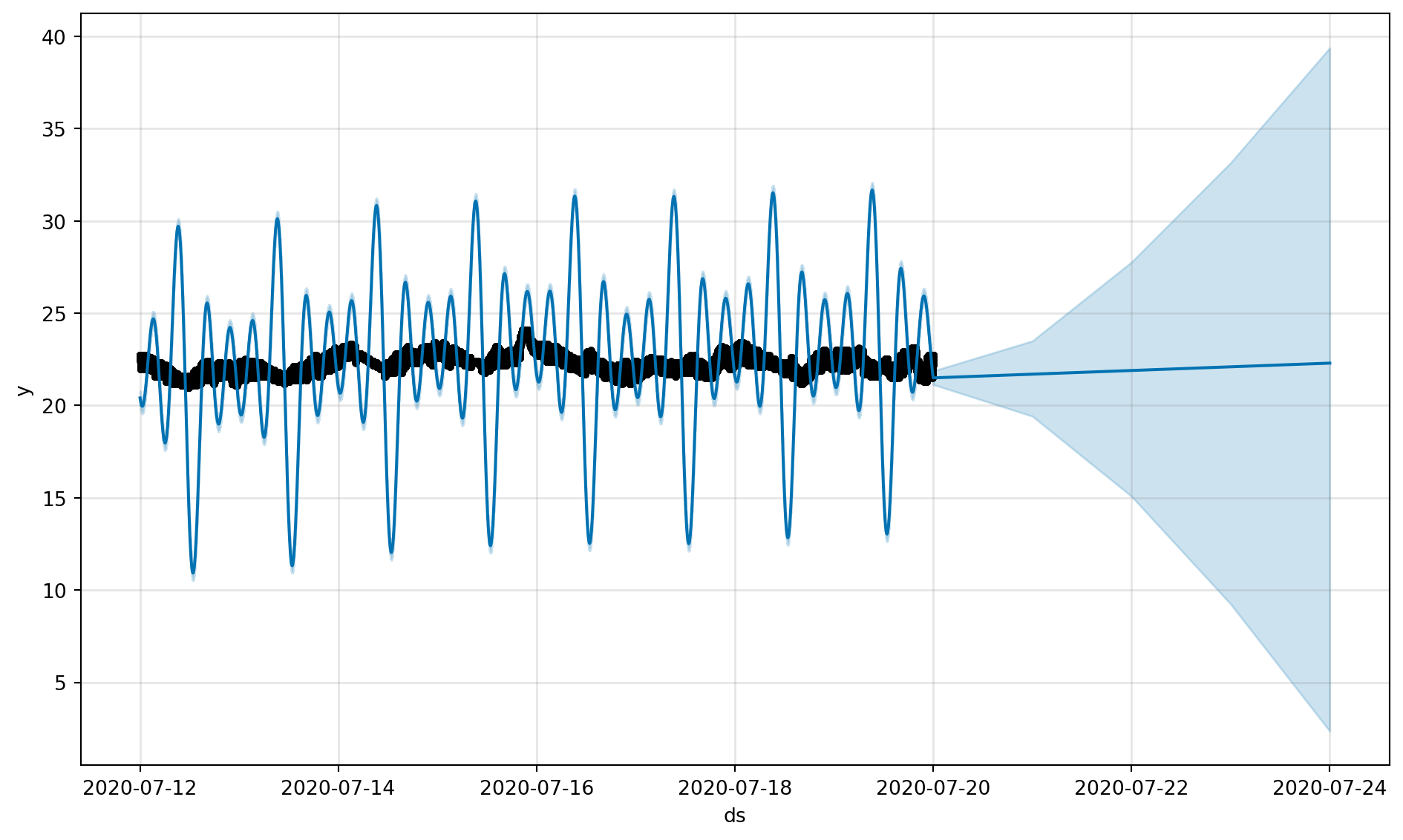
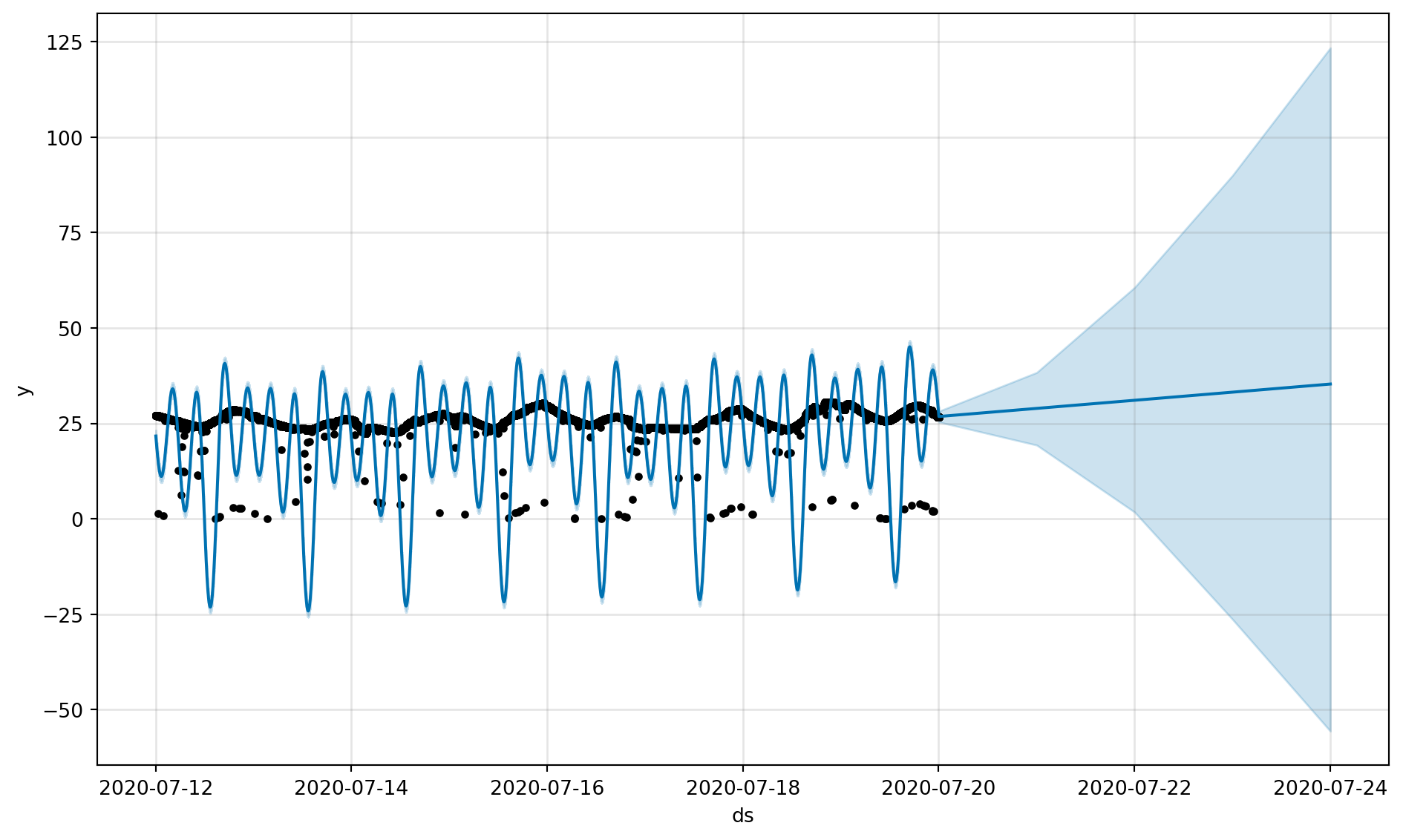
def get_forecast_data(df):
    device_df = df.select(pl.col(["timestamp", "temp"])).rename({"timestamp":"ds", "temp":"y"})
    device_df = device_df.to_pandas()
    m = Prophet()
    m.fit(device_df)

    future = m.make_future_dataframe(periods=4)
    forecast = m.predict(future)
    forecast[['ds', 'yhat', 'yhat_lower', 'yhat_upper']].tail()
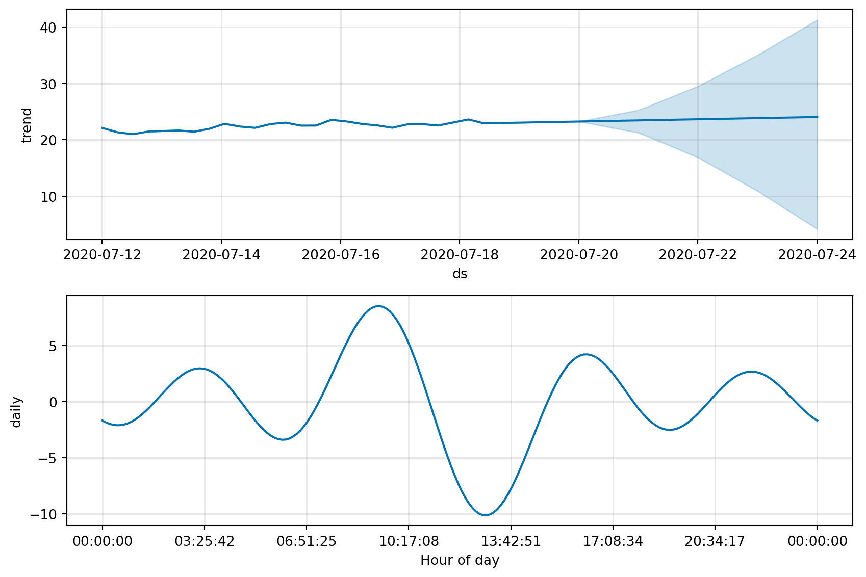
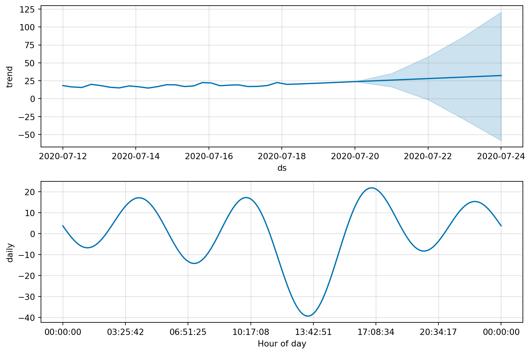
    fig = m.plot(forecast)
    fig_comp = m.plot_components(forecast)
    #fig_dyplot = dyplot.prophet(m, forecast)
    #fig_dyplot.show()
    return fig, fig_comp

fig, fig_comp = get_forecast_data(df_device_1)
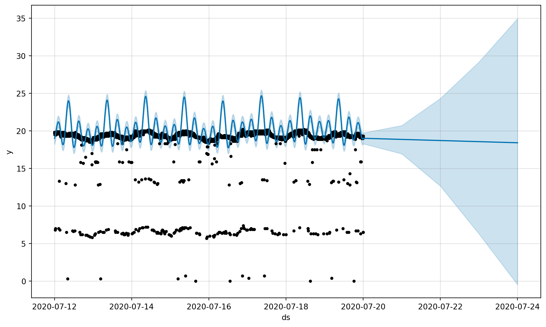
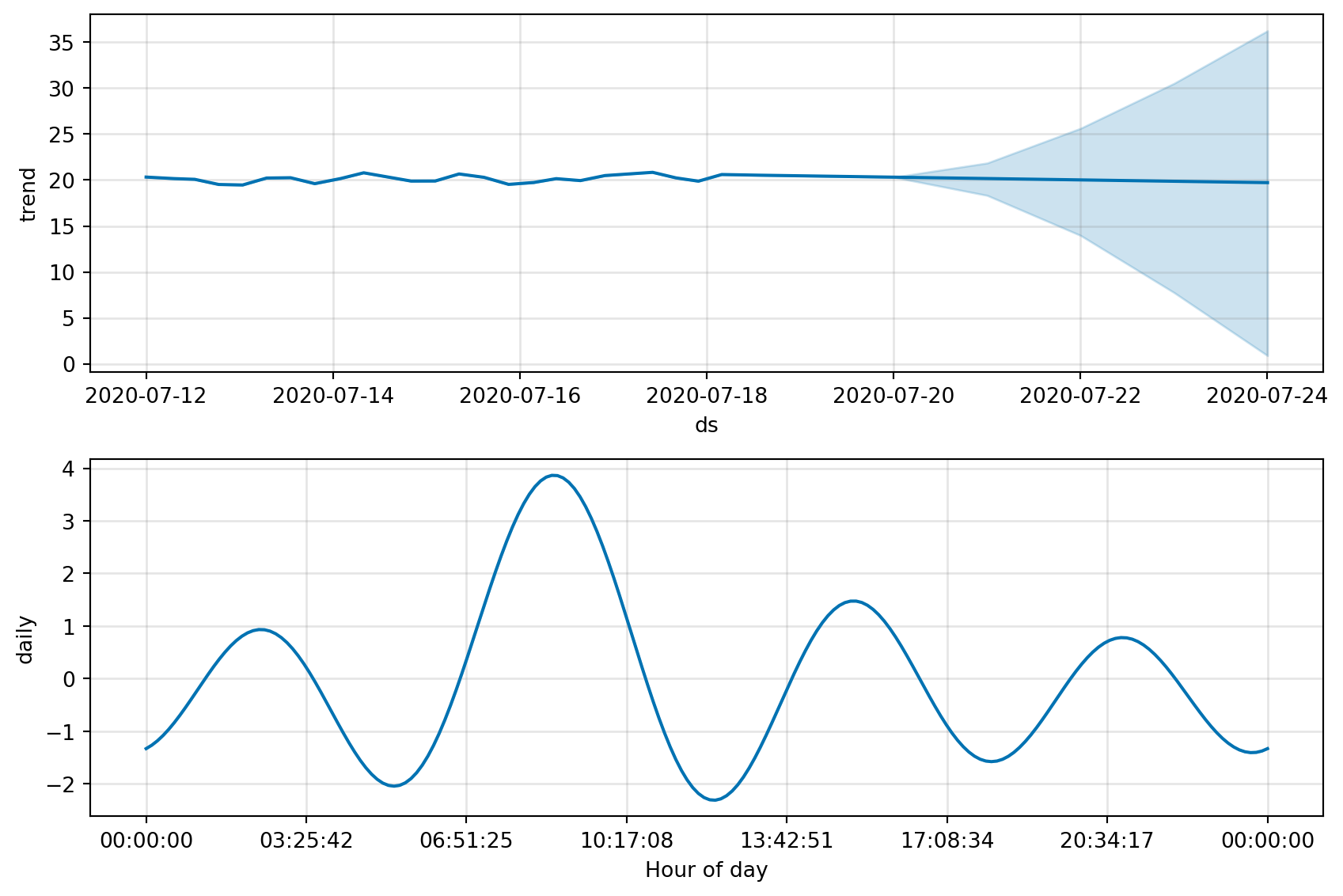
fig, fig_comp = get_forecast_data(df_device_2)
fig, fig_comp = get_forecast_data(df_device_3)

21:45:04 - cmdstanpy - INFO - Chain [1] start processing
21:46:24 - cmdstanpy - INFO - Chain [1] done processing
21:46:45 - cmdstanpy - INFO - Chain [1] start processing
21:47:28 - cmdstanpy - INFO - Chain [1] done processing
21:47:41 - cmdstanpy - INFO - Chain [1] start processing
21:48:40 - cmdstanpy - INFO - Chain [1] done processing